The next package release into AWS Athena

RBloggers|RBloggers-feedburner
RAthena 1.7.1 and noctua 1.5.1 package versions have now been released to the CRAN. They both bring along several improvements with the connection to AWS Athena, noticeably the performance speed and several creature comforts.
These packages have both been designed to reflect one another,even down to how they connect to AWS Athena. This means that all features going forward will exist in both packages. I will refer to these packages as one, as they basically work in the same way.
Performance improvements:
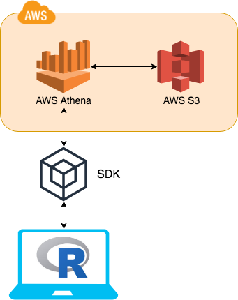
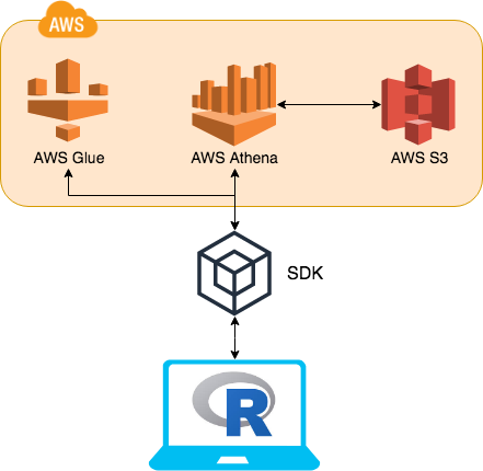
Initially the packages utilised AWS Athena SQL queries. This was to achieve all the functional requirements of the DBI package framework. However the package would always send a SQL query to AWS Athena which in turn would have to lift a flat file from AWS S3, before returning the final result to R. This means the performance of the packages would be limited and fairly slow compared to other data base backends.

The biggest change is the adoption of more functionality of the SDKs (software development kit) into AWS. The key component that has been adopted is AWS Glue. AWS Glue contains all of AWS Athena table DDL’s. This means instead of going to AWS Athena for this information AWS Glue can be used instead.

By utilising AWS Glue, the table meta data (column names, column types, schema hierarchy etc…) can easily be retrieved at a fraction of the time it would of taken to query AWS Athena. Previously the DBI function dbListTables would send a query to AWS Athena, this would retrieve all the tables listed in all schemas. This would take over 3 seconds. Now using AWS Glue to retrieve the same data, it takes less than 0.5 of a second.
dplyr
When AWS Glue is used to collect metadata around a table in AWS Athena, a performance in dplyr::tbl can be done. I would like to say thanks to @OssiLehtinen for developing the initial implementation as this improvement would have been overlooked.
dplyr::tbl has two key methods when creating the initial object. The first is called SQL identifiers and this is the method that benefits from the new AWS Glue functionality. To use SQL identifiers is fairly straight forward.
library(DBI)
library(dplyr)
library(RAthena) #Or library(noctua)

con = dbConnect(athena())

dbWriteTable(con, "iris", iris)

ident_iris = tbl(con, "iris")
dplyr can identify the iris table within the connected schema. When a user uses the SQL identifier method in dplyr::tbl, AWS Glue is called to retrieve all the meta data for dplyr. This increases the performance from 3.66 to 0.29 seconds. The second method is called SQL sub query. This unfortunately won’t benefit from the new feature and will run in slower at 3.66 seconds.
subquery_iris = tbl(con, sql("select * from iris"))
Therefore I recommend the use of SQL identifier method when using dplyr's interface.
Creature Comforts
AWS Athena Metadata
Due to user feature requests the packages now return more meta data around each query sent to AWS Athena. Thus the basic level of meta data returned, is the amount of data scanned by AWS Athena. This is formatted into a readable format depending on the amount of data scanned.
library(DBI)
library(RAthena) #Or library(noctua)

con = dbConnect(athena())

dbWriteTable(con, "iris", iris)

dbGetQuery(con, "select * from iris")
Info: (Data scanned: 860 Bytes)
     sepal_length sepal_width petal_length petal_width   species
  1:          5.1         3.5          1.4         0.2    setosa
  2:          4.9         3.0          1.4         0.2    setosa
  3:          4.7         3.2          1.3         0.2    setosa
  4:          4.6         3.1          1.5         0.2    setosa
  5:          5.0         3.6          1.4         0.2    setosa
 ---
146:          6.7         3.0          5.2         2.3 virginica
147:          6.3         2.5          5.0         1.9 virginica
148:          6.5         3.0          5.2         2.0 virginica
149:          6.2         3.4          5.4         2.3 virginica
150:          5.9         3.0          5.1         1.8 virginica
However if you set the new parameter statistics to TRUE then all the metadata around that query is printed out like so:
dbGetQuery(con, "select * from iris", statistics = TRUE)
$EngineExecutionTimeInMillis
[1] 1568

$DataScannedInBytes
[1] 860

$DataManifestLocation
character(0)

$TotalExecutionTimeInMillis
[1] 1794

$QueryQueueTimeInMillis
[1] 209

$QueryPlanningTimeInMillis
[1] 877

$ServiceProcessingTimeInMillis
[1] 17

Info: (Data scanned: 860 Bytes)
     sepal_length sepal_width petal_length petal_width   species
  1:          5.1         3.5          1.4         0.2    setosa
  2:          4.9         3.0          1.4         0.2    setosa
  3:          4.7         3.2          1.3         0.2    setosa
  4:          4.6         3.1          1.5         0.2    setosa
  5:          5.0         3.6          1.4         0.2    setosa
 ---
146:          6.7         3.0          5.2         2.3 virginica
147:          6.3         2.5          5.0         1.9 virginica
148:          6.5         3.0          5.2         2.0 virginica
149:          6.2         3.4          5.4         2.3 virginica
150:          5.9         3.0          5.1         1.8 virginica
This can also be retrieved by using dbStatistics:
res = dbExecute(con, "select * from iris")

# return query statistic
query_stats = dbStatistics(res)

# return query results
dbFetch(res)

# Free all resources
dbClearResult(res)
RJDBC inspired function
I have to give full credit to the package RJDBC for inspiring me to create this function. DBI has got a good function called dbListTables that will list all the tables that are in AWS Athena. However it won’t return to which schema each individual table is related to. To over come this RJDBC has a excellent function called dbGetTables. This function returns all the tables from AWS Athena as a data.frame. This has the advantage of detailing schema, table and table type. With the new integration into AWS Glue this can be returned quickly.
dbGetTables(con)
      Schema             TableName      TableType
 1:  default             df_bigint EXTERNAL_TABLE
 2:  default                  iris EXTERNAL_TABLE
 3:  default               mtcars2 EXTERNAL_TABLE
 4:  default         nyc_taxi_2018 EXTERNAL_TABLE
This just makes it a little bit easier when working in different IDE’s for example Jupyter.
Backend option changes
This is not really a creature comfort but it still interesting and useful. Both packages are dependent on data.table to read data into R. This is down to the amazing speed data.table offers when reading files into R. However a new package, with equally impressive read speeds, has come onto the scene called vroom. As vroom has been designed to only read data into R similarly to readr, data.table is still used for all of the heavy lifting. However if a user wishes to use vroom as the file parser an *_options function has been created to enable this:
nocuta_options(file_parser = c("data.table", "vroom"))

# Or

RAthena__options(file_parser = c("data.table", "vroom"))
By setting the file_parser to vroom then the backend will change to allow vroom's file parser to be used instead of data.table.
If you aren’t sure whether to use vroom over data.table, I draw your attention to vroom boasting a whopping 1.40GB/sec throughput.
Statistics taken from vroom’s github readme
| package | version | time (sec) | speed-up | throughput |
|---|---|---|---|---|
| vroom | 1.1.0 | 1.14 | 58.44 | 1.40 GB/sec |
| data.table | 1.12.8 | 11.88 | 5.62 | 134.13 MB/sec |
| readr | 1.3.1 | 29.02 | 2.30 | 54.92 MB/sec |
| read.delim | 3.6.2 | 66.74 | 1.00 | 23.88 MB/sec |
RStudio Interface!
Due to the ability of AWS Glue to retrieve metadata for AWS Athena at speed, it has now been possible to add the interface into RStudio’s connection tab. When a connection is established:
library(DBI)
library(RAthena) #Or library(noctua)

con = dbConnect(athena())
The connection icon will as follows:

The AWS region you are connecting to will be reflected in the connection (highlighted above in the red square). This is to help users that are able to connect to multiple different AWS Athena over different regions.
Once you have connected AWS Athena, schema hierarchy will be displayed. In my example you can see some of the tables I have created when testing these packages.

For more information around RStudio’s connection tab please check out RStudio preview connections.
Summary
To sum up, the Rathena and noctua latest versions have been released to cran with all the new goodies they bring. As these packages are based on AWS SDK’s they are highly customisable. Features can easily be added to improve the packages when connecting to AWS Athena. So please raise any feature requests / bug issues to: https://github.com/DyfanJones/RAthena and https://github.com/DyfanJones/noctua
